We have seen on-policy and off-policy RL algorithms, but there is a problem: tabular MDP / RL methods are polynomial in the number of actions \(\lvert A \rvert\) and states \(\lvert X \rvert\). The goal now is to scale from simple tabular RL to large \(\lvert A \rvert\) and \(\lvert X \rvert\). To do so, we need to extend model-free methods such as TD-learning and Q-learning to large state and action spaces.

The only way to do this is to learn approximations of value functions (through regression).

The first step is to recast tabular RL as an optimisation problem.

1. Tabular RL as an optimisation problem

We re-interpret the model-free methods from the previous chapter — TD- and Q-learning — as optimisation problems where each iteration is a single gradient update.

Consider TD-learning:

This is the update rule of an optimisation algorithm. We just have to parametrise the estimate of \(V^{\pi}\) with parameters \(\theta\) and update them according to the gradient of some loss. In a finite domain (e.g. tabular), we can parametrise the value function with a separate parameter for each state:

To re-derive the \(V^{\pi}\) update as a gradient update we need a loss function. Consider

and using the Bellman equation,

which is the classical squared loss between the parameter and the target label \(v^{\pi}\). Now we can view TD-learning as SGD. The first issue is that we cannot compute the expectation, so as in TD-learning we use a bootstrapped estimate of \(V^{\pi}\). This bootstrapped estimate is treated as if it were independent of the current \(\theta\):

where \(\theta_{\text{old}} = \theta\) but is treated as a constant w.r.t. \(\theta\). Bootstrapping thus means using “old” value estimates as labels.

Secondly, the expectation is over the transition model — which we are trying to avoid in model-free methods — so we use a Monte Carlo estimate from a single sample. This is only possible because transitions are conditionally independent given the state–action pair.

Using these shortcuts, the loss becomes

with gradient w.r.t. \(\theta(x)\):

This is the temporal-difference (TD) error: it compares the previous estimate of the value function to the bootstrapped one.

Model free

2. Value function approximation

Now that we have the value-function update as a gradient step, it is natural to find an approximation of the parametrised \(V(x; \theta)\) or \(Q(x, a; \theta)\) to scale to large settings. Think of this as a regression problem mapping state(–action) pairs to a real number. This is a strict generalisation of the tabular setting, where we used a separate parameter per state–action pair.

For large state–action spaces, we exploit smoothness (the value function takes similar values in similar states) to compress the representation. An easy way to do this is linear function approximation, e.g. for \(Q\):

where \(\phi\) is a hand-designed feature map. (A common alternative is to use a NN to learn these features — deep reinforcement learning.)

After observing a transition \((x, a, r, x')\), the gradient update (analogous to the one for \(V\)) uses

The difference between the current approximation and the optimisation target,

is called the Bellman error. Analogously to TD-learning, we obtain the gradient update

and in the linear case

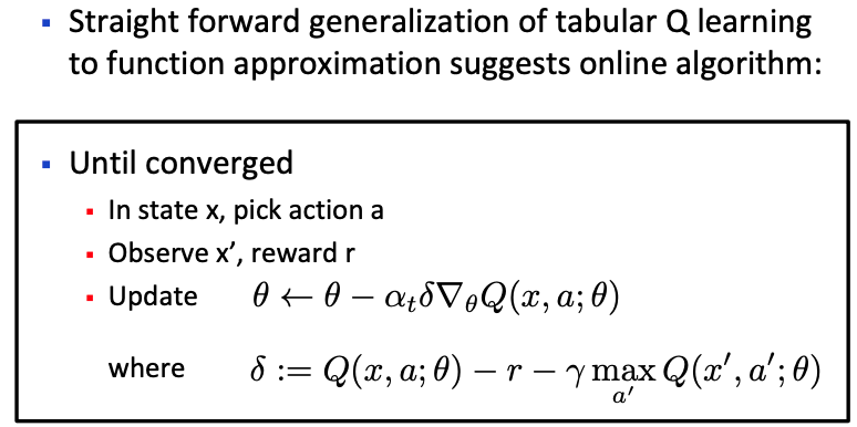
But this algorithm is rather slow!

3. Neural Fitted Q-iteration / DQN

To accelerate Q-learning with (neural) function approximation:

• use “experience replay” — maintain a dataset \(D\) of observed transitions;
• clone the network to keep “target” values constant across episodes (the cloned network is the target network \(Q(x', a'; \theta^{\text{old}})\)).

The loss is then

How exactly this is implemented varies.

Increasing stability — Double DQN

Standard DQN suffers from maximisation bias: since we max over \(Q\), which is itself an estimate, we can get over-estimates. The idea is to split the max: Double DQN uses the current network to evaluate the argmax (action selection), then evaluates that action with the cloned target network:

where

The fundamental idea of Q-learning is that it chooses the next action by implicitly defining a policy via

but this is intractable for large or continuous action spaces.

4. Policy search methods

Learn a parametrised policy (actor): \(\pi(x) = \pi_{\theta}(x) = \pi(x; \theta)\). For episodic tasks (when the agent can be reset), expected rewards can be computed by “rollouts” (Monte Carlo forward sampling — on-policy). The idea is to find optimal parameters via global optimisation:

4.1 Policy gradients

The objective is to maximise

How do we obtain gradients w.r.t. \(\theta\)?

Proof. Recall

Then

Exploiting the MDP structure. To obtain gradients of \(J(\theta)\) we need to compute

From the MDP, \(r(\tau) = \sum_{t=0}^{T} \gamma^t r(x_t, a_t)\), and the trajectory distribution factorises as

Taking the gradient of the log-probability,

Since the dynamics and initial-state distribution do not depend on \(\theta\), \(\nabla_{\theta} \log p(x_0) = 0\) and \(\nabla_{\theta} \log p(x_{t+1} \mid x_t, a_t) = 0\). Therefore

Thus

Although these gradients are unbiased, they have very large variance. We can reduce this variance using baselines.

Proof. It suffices to show \(\mathbb{E}_{\tau \sim \pi_{\theta}}[b\, \nabla \log \pi_{\theta}(\tau)] = 0\). Using \(\nabla_{\theta} \log \pi_{\theta}(\tau) = \nabla_{\theta} \pi_{\theta}(\tau) / \pi_{\theta}(\tau)\),

Example: baseline = downstream return. A state-dependent baseline:

This baseline subtracts the returns of all actions before time $t$. Intuitively, the score gradient then only considers downstream returns. We obtain the estimator

where \(G_t\) is the (bounded) discounted payoff from time \(t\): the reward-to-go following action \(a_t\). Also called the (bounded) downstream return:

Performing SGD with the score gradient and downstream returns is the REINFORCE algorithm (Williams, 1992):

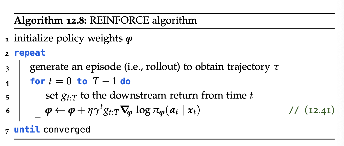
(Initialise the policy parameters, set \(G_t\) to the return from step \(t\), and update.)

The variance of REINFORCE can be reduced further. The basic estimate is

A common variance-reduction trick is a stronger baseline \(b_t\):

One example is the mean over returns:

Remark. The big advantage of policy-gradient methods is that they work in continuous action spaces. However, REINFORCE is not guaranteed to find an optimal policy — even in very small domains it can get stuck in local optima.

Next, we combine value approximation (Q-learning) and policy gradient methods, leading to the more practical family of actor–critic methods.

5. On-policy: actor–critic methods

Actor–critic methods reduce the variance of policy-gradient estimates by using ideas from value-function approximation.

Idea: use function approximation both for value functions and for policies.

It has an important property — for the greedy action,

The Bellman optimality principle is essentially: the max is always at least the average — a policy is optimal iff there is no advantage in any state:

The greedy policy can be re-stated as \(\pi_G(x) = \operatorname{argmax}_a Q^{\pi}(x, a) = \operatorname{argmax}_a A^{\pi}(x, a)\).

We have already seen how to estimate the value function; below we will see we can also estimate it off-policy.

5.1 Policy Gradient Theorem

Recall from §4.1 how to compute policy gradients with the canonical MC-based score-function trick (REINFORCE). We derived

As mentioned, this is slow, so we try to predict the reward-to-go using ideas from value-function estimation. This leads to the actor–critic family. We state the Policy Gradient Theorem, the basis of these methods.

5.1.1 Reinterpreting score gradients

We want to rewrite the gradient to bring the value function back into play, so we can approximate both the value and the policy and trade off bias against variance:

Using nested expectations:

(the inner expectation is over \((r_t, x_{t+1}, a_{t+1}, r_{t+1}, \ldots)\))

We can rewrite this as a single integral using the occupancy measure:

where \(\rho_{\theta}\) is the discounted state occupancy measure (an unnormalised distribution):

(There are many variants of the PGT; we derived the one for infinite-horizon discounted payoffs.) Abusing notation,

This is the Policy Gradient Theorem. The idea is to plug in an approximation of the state–action value function, \(Q(x, a; \theta_Q)\).

Summary. Actor–critic algorithms combine:

• an Actor (parametrised policy);
• a Critic (value-function approximation).

In Deep RL, both approximations are NNs.

5.2 Online actor–critics

Many algorithms can be derived from the Policy Gradient Theorem above. The main ones combine value-function approximation (critic) with the policy-gradient method, approximating

How do we update the critic? TD-learning (online setting). Subtracting a state-dependent baseline doesn’t change the expectation; one common choice is the value function:

With the advantage estimate

we get

i.e. the A2C algorithm.

Everything we have discussed is very on-policy. Next we move to still on-policy methods that allow bigger updates, and then to off-policy algorithms.

5.3 TRPO & PPO

The idea is faster optimisation:

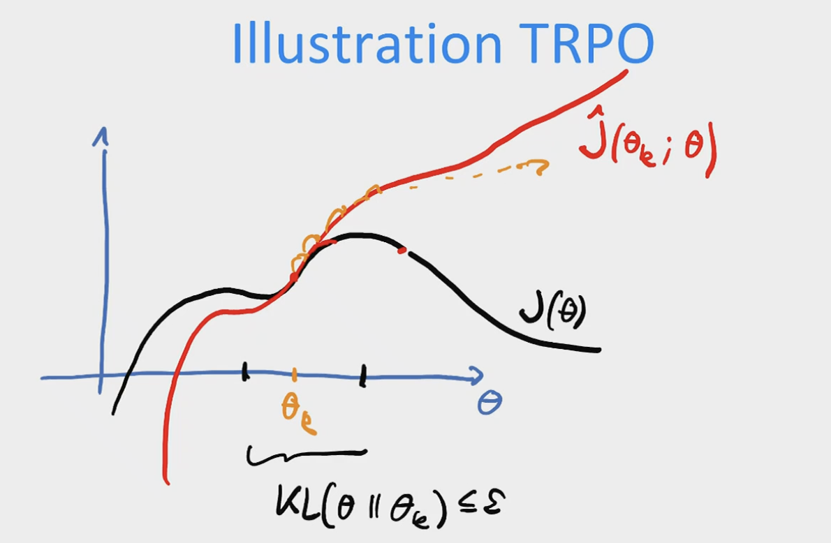
The basic idea is to build a trust region in which we can re-use data via importance sampling:

This is the basic idea of TRPO:

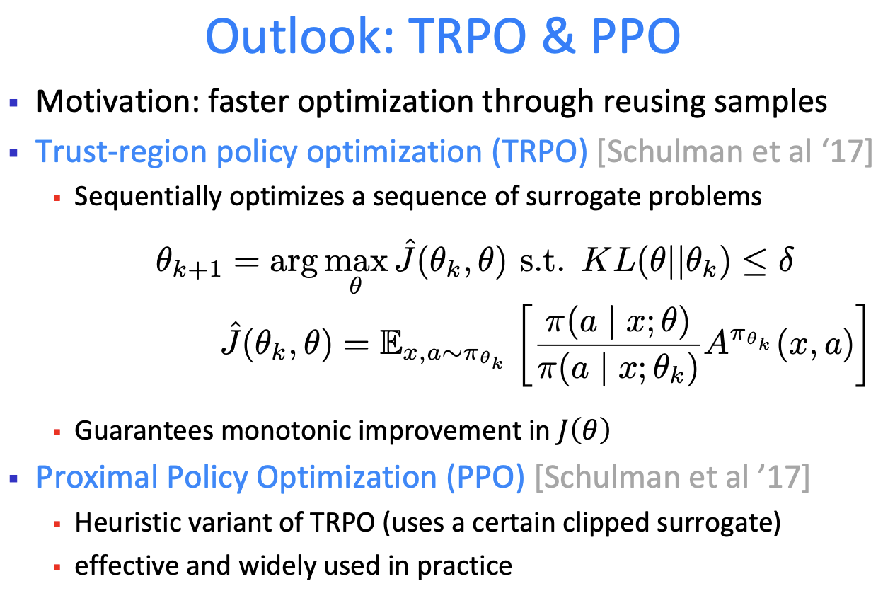
(See tutorials.) It’s a little bit off-policy, but still on-policy. Now we transition to genuinely off-policy methods.

5.4 Another approach to policy gradients

Starting point: not REINFORCE, but Q-learning used for off-policy methods (DQN). The motivation was the intractability of \(L(\theta)\), which required computing \(\max_{a'} Q(x', a'; \theta^{\text{old}})\). One thing we can do is use an actor — a parametrised policy — to predict that greedy action. So we use a new NN \(\pi(x'; \theta_{\pi})\): we want to follow the greedy policy

If we allow rich enough policies, this is equivalent to

where \(\mu(x) > 0\) “explores all states”. The idea is to apply SGD to this objective; we just need differentiable approximations of \(Q\) and \(\pi\) (i.e. NNs).

Computing the gradients. Given the objective above, the chain rule gives

But there is an issue: policy-gradient methods rely on randomised policies for exploration; this method uses deterministic policies. How do we ensure sufficient exploration?

Since the method is off-policy, we can inject additional action noise (e.g. Gaussian) to encourage exploration (akin to \(\varepsilon\)-greedy).

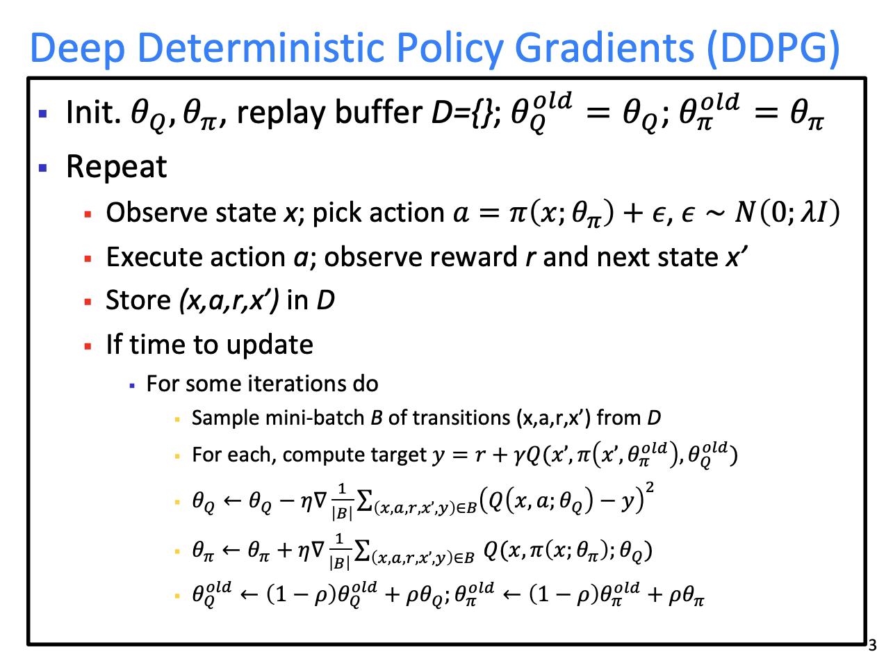
One issue is over-confidence — overestimation bias.

TD3

Twin Delayed DDPG: uses two critic networks and evaluates the target with the smaller of the two.

6. Randomised policies

Can we, instead of injecting random noise, ensure exploration by directly allowing randomised policies?

For the critic update:

where

We can obtain unbiased gradient estimates by sampling \(a' \sim \pi(\cdot \mid x'; \theta_{\pi}^{\text{old}})\). What about the policy update? Recall, for deterministic policies:

If we instead want

assume Gaussian policies \(a \sim \mathcal{N}(\mu_{\theta_{\pi}}, \Sigma_{\theta_{\pi}})\). We can reparametrise as

Plugging into (1):

The resulting algorithm is called SVG (Stochastic Value Gradients). (See variational inference notes.)

7. RL as inference: entropy-regularised RL

One way to do this is to introduce binary variables \(\mathcal{O}_t \in \{0, 1\}\), with \(\mathcal{O}_t = 1\) denoting that \(a_t\) was optimal. We define a likelihood relating the state, action and optimality variable to the exponentiated reward:

The temperature \(\lambda\) controls the peakedness — a small \(\lambda\) strongly favours actions with large rewards.

With this setup, we can think about the conditional probability over trajectories in the underlying MDP. Conditioning on \(\mathcal{O}_t = 1\) for all \(t \in \{1, \ldots, T\}\):

This is a complicated distribution, but we can approximate it (using variational inference) with a policy we can implement. Use a parametrised policy as a variational posterior:

This induces a distribution over trajectories under \(\pi_{\theta}\):

from which we can sample. How do we pick \(\pi_\theta\) to bring these distributions close? With the KL divergence — view inference as

This is equivalent to maximising the entropy-regularised RL objective:

Interpretation.

• The policy \(\pi_{\theta}\) is trained to approximate the posterior over optimal trajectories.
• The entropy term \(H[\pi_{\theta}(\cdot \mid x_t)]\) arises naturally from KL minimisation, rather than being added by hand.
• The temperature \(\lambda\) controls the reward–entropy trade-off.

This entropy-regularised approach is a natural way to encourage exploration in MDPs:

This suitably defines regularised (action-)value functions, called soft value functions. One can derive the same kind of algorithm as before (SVG), now with action entropy: the resulting algorithm is SAC: Soft Actor-Critic — the same as SVG, but encouraging some entropy in the action distribution. SAC is one of the most common off-policy actor–critic methods in use.

A closely related approach replaces entropy regularisation with a KL constraint (MPO): updates the policy by fitting it to a target soft distribution

From entropy to KL regularisation. So far we have discussed

A closely related problem:

Instead of maximising entropy directly, we regularise the policy with a KL divergence to a reference (pretrained) policy \(\pi_{\text{ref}}\), maintaining proximity to it.