“An agent navigating through MDPs”. The difference from the previous chapters is that in RL the policy can be randomised, and the dynamics are unknown. Reinforcement learning is concerned with probabilistic planning in unknown environments.

The crucial trade-off in RL is exploration vs. exploitation, as in Bayesian Optimisation (BO). The agent must decide whether it is better to explore and learn about the environment, or to exploit current knowledge to maximise reward.

In fact, BO can be seen as RL with a fixed state and continuous action space: in BO we used regret as a performance metric (minimising regret corresponds to maximising reward).

Before delving into RL definitions, recall what is different in RL from standard supervised learning:

• Data is not i.i.d.;
• The data we receive depends on our actions;
• Some actions yield higher rewards than others.

But what is “data” in RL? Data is collected dynamically from the environment, so it consists of trajectories.

Data

Settings

Data collection is commonly classified into three settings:

1. Episodic setting: the agent performs a sequence of “training” rounds (called episodes); after each, the environment resets.
2. Continuous setting (non-episodic): the agent learns online, producing a single trajectory.
3. Offline setting: the agent must learn from a fixed dataset — a “library” of pre-recorded trajectories.

Policy method

Another important distinction is how data is collected:

1. On-policy (learning by doing — and only from what you just did): the agent updates the policy using only data collected with the current policy (e.g. SARSA, PPO).
2. Off-policy (learning by watching others or your past self): the target policy (the one being learned) is different from the behaviour policy (the one used to generate the data); these methods are typically more sample-efficient (e.g. Q-learning, DQN).

Model approach

There are two fundamental approaches to RL:

1. Model-based RL: aim to learn the underlying MDP. We estimate (learn) the transition probabilities \(p\) and the reward function \(r\).
2. Model-free RL: aim to learn the value function directly.

We begin with model-based methods.

Model-based approach

We don’t know how the world works, so we try to “build a map” (a model) of it from the data we’ve collected.

Learning the MDP

We need to estimate the transition probabilities and the reward function:

To pick parameters that maximise the expected reward, we apply Maximum Likelihood Estimation (MLE) to the observed data. We treat each transition \(x' \mid x, a\) as a sample from a categorical random variable and estimate its probabilities. Under the Markov assumption, estimating the transition probabilities reduces to a frequency count:

where the numerator counts the number of transitions from \(x\) to \(x'\) when playing action \(a\). Similarly, the MLE of the reward is

How do we handle the exploration–exploitation dilemma here?

Exploration vs. exploitation dilemma

Given the current model, how do we choose actions? If we stick to exploitation we may get stuck in a sub-optimum; if we keep choosing actions at random, we will eventually estimate all probabilities and rewards correctly, but we’ll perform poorly along the way.

So it really depends on the setting, but a good balance is achievable with “$\varepsilon$-greedy”.

\(\varepsilon\)-greedy

The simplest idea for a balance. At each time step \(t\) we throw a biased coin. If it lands heads, we pick an action uniformly at random (exploration); if tails, we pick the best action under the current model (exploitation). The probability of heads at time \(t\) is \(\varepsilon_t\).

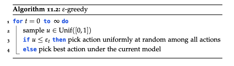
This is a general framework for trading off exploration and exploitation. Surprisingly, this simple algorithm works well in practice.

Optimism

Recall from the multi-armed bandit problem that a key principle for trading off exploration and exploitation is optimism in the face of uncertainty. Applied to RL: assume the dynamics and reward estimates work in our favour — i.e. our estimates are at least as optimistic as the truth.

We look for optimistic estimates of \(p, r\), yielding an optimistic underlying MDP biased towards exploration. The rewards from this MDP are upper bounds on the true rewards.

Technically, if \(r\) and \(p\) are unknown, we set

i.e. the maximum reward an agent can get and the probability of staying in the fairy-tale state \(x^{*}\).

In practice, the decision of when the estimates are good enough has to be tuned.

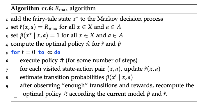
How many transitions do we need for good enough \(p, r\) estimates? We use Hoeffding’s inequality: treating the transitions and rewards as conditionally independent, the inequality tells us that for the absolute approximation error to be below \(\epsilon\) with probability at least \(1 - \delta\), we need

This yields the following theorem:

Challenges of the model-based approach

1. Memory: We must store all parameters; for each \(x, a, x'\) we store \(p\) and \(r\). In the tabular setting this is \(O(n^2 m)\).
2. Computation time: We must repeatedly solve the estimated MDP: \(O(nm)\) per iteration.

Model-free approach

Model-free methods estimate the value function directly. They do not need to remember the underlying MDP — only the value (or policy).

On-policy value estimation

Suppose the agent uses a fixed policy \(\pi\). Then we can estimate the value function as before:

A first idea is to estimate it via Monte Carlo. MC produces an unbiased estimate but requires complete trajectories, and the right-hand side still depends on \(v^{\pi}\) itself. The key idea is to use a bootstrapping estimate of the value function instead. Bootstrapping is a core concept of model-free RL; it generally produces biased estimates, but with much lower variance and faster updates.

One way to compute the value-function update from samples is to mix new estimates with previous estimates using a learning rate \(\alpha_{t}\). This yields the temporal-difference (TD) algorithm:

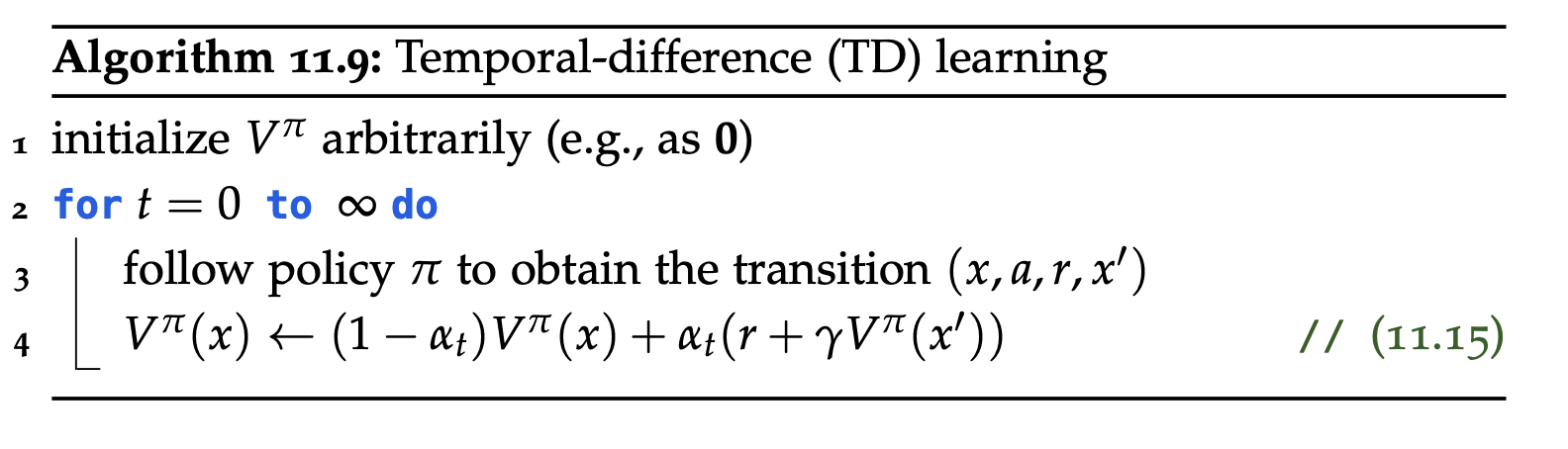
(We use a lookup table for the values given the state.)

SARSA

On-policy

Off-policy

Off-policy value estimation

At state \(x\), pick an action \(a\) to obtain a transition \((x, a, r, x')\). Then update the value estimate using bootstrapping:

As for the on-policy case, we have the convergence theorem:

Remark: this is off-policy because action \(a\) does not need to be picked following \(\pi\).

Optimal value estimation

Recall that:

1. The optimal value function \(V^{*}(x)\) induces the optimal policy \(\pi^{*}\).
2. For the optimal value function, \(V^{*}(x) = \max_a Q^{*}(x, a)\), where \(Q^{*}(x, a) = r(x, a) + \gamma \sum_{x'} P(x' \mid x, a)\, V^{*}(x')\).

So the idea is to estimate \(Q^{*}(x, a)\) directly from samples. Below are some of the most common ways to do so.

1) Q-learning

Suppose we have an initial estimate \(\hat{Q}^{*}(x, a)\) and observe a transition \((x, a, x')\) with reward \(r\). The update is

How do we handle the exploration–exploitation trade-off? Two options:

• \(\varepsilon\)-greedy;
• optimistic exploration.

1.1 Convergence of optimistic Q-learning

Similar to R_max: initialise

and at time \(t\) pick \(a_t \in \operatorname{argmax}_a \hat{Q}^{*}(x_t, a)\).

Properties:

• Memory: store \(\hat{Q}^{*}(x, a)\) for each \((x, a)\) — \(O(n \cdot m)\).
• Computation time: \(O(m)\) per iteration to compute \(\operatorname{argmax}_a \hat{Q}(x_t, a)\).

Neural Fitted Q-iteration / DQN

To accelerate Q-learning with (neural) function approximation:

• use “experience replay” — maintain a dataset \(D\) of observed transitions;
• clone the network to maintain constant “target” values across episodes.

The fundamental idea of Q-learning is that it chooses the next action by implicitly defining a policy via

but this is intractable for large or continuous action spaces.

Policy search methods

Learn a parametrised policy (actor): \(\pi(x) = \pi_{\theta}(x) = \pi(x; \theta)\). For episodic tasks (i.e. when the agent can be reset), expected rewards can be computed by “rollouts” (Monte Carlo forward sampling — on-policy). The idea is to find optimal parameters via global optimisation: