Model-Based Approximate RL
Contents
In model-based RL we want to learn the model of the environment, i.e. the transition probabilities and the reward function. We can then use the learned model to plan a new policy \(\pi\).
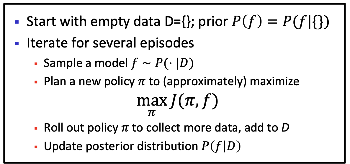
We typically start with a policy \(\pi\) and some initial dataset \(D\). We iterate over many episodes: collect data from \(\pi\), estimate \(p, r\), then plan a new policy based on the estimated model.
So we cover:
- planning;
- learning \(f, r\);
- the trade-off between exploration and exploitation.
Planning
We focus on planning in continuous, fully observed state spaces with non-linear transitions, without constraints.
Planning with a known deterministic model
Assume we have a known deterministic model for the dynamics:
\[x_{t+1} = f(x_t, a_t).\]The objective is
\[\max_{a_{0:\infty}}\, \sum_{t = 0}^{\infty} \gamma^t r(x_t, a_t) \quad \text{s.t.} \quad x_{t+1} = f(x_t, a_t).\]Since we are optimising over an infinite horizon, this problem cannot be solved directly.
MPC: model-predictive control / RHC
Solution: plan over a finite horizon $H$, carry out the first action, then re-plan.
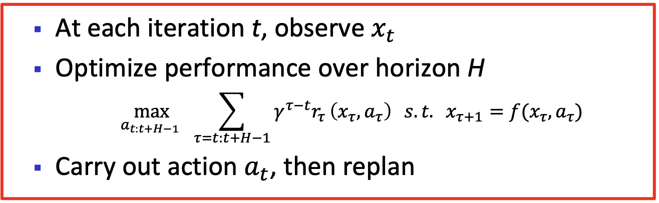
So at each iteration we solve an optimisation problem. For deterministic models \(f\), \(x_{\tau}\) is determined by \(a_{t:\tau-1}\):
\[x_{\tau} := x_{\tau}(a_{t:\tau - 1}) = f(\,f(\,\ldots f(\,f(x_t, a_t),\, a_{t+1})\, \ldots,\, a_{\tau - 1}\,)\,).\]So at each step we maximise
\[J_H(a_{t:t+H-1}) := \sum_{\tau = t}^{t+H-1} \gamma^{\tau - t}\, r\!\left(x_{\tau}(a_{t:\tau - 1}),\, a_{\tau}\right).\]How do we optimise this? For continuous actions we can analytically compute gradients (BPTT), but it’s challenging — so we usually use heuristic global optimisation.
Example — **random shooting**: a sampling approach for global optimisation of \(J_H\). Generate $m$ sets of random samples \(a^{i}_{t:t+H-1}\) and pick the sequence that optimises:
\[i^{*} = \operatorname{argmax}_{i \in \{1, \ldots, m\}} J_H(a^{i}_{t:t+H-1}).\]Limitation: a common problem of finite-horizon methods is that, in sparse-reward settings, there is often no signal to follow.
Remark. If we use the value estimate \(V\), then for \(H = 1\) maximising \(J_H\) coincides with the **greedy policy** w.r.t. \(V\):
\[a_t := \operatorname{argmax}_{a \in \mathcal{A}} \hat{J}_1 = \text{greedy policy}.\]MPC for stochastic transition models
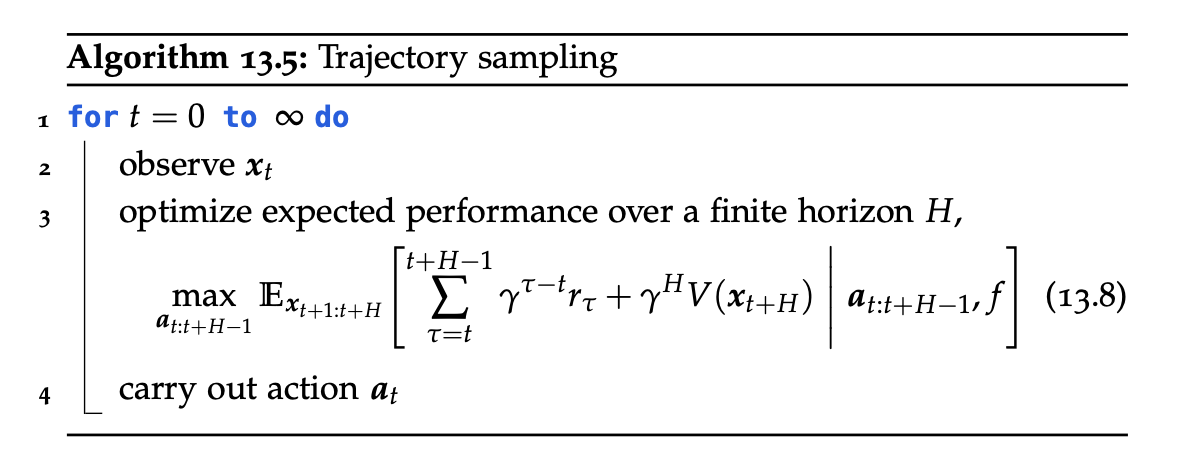
For probabilistic transition models, MPC requires optimising:

Computing this expectation exactly requires solving a high-dimensional integral.
Monte Carlo trajectory sampling
A common approach: Monte Carlo trajectory sampling.
Learning
Due to the Markovian structure of the MDP, observed transitions and rewards are (conditionally) independent. If we don’t know the dynamics and reward, we can estimate them off-policy with standard supervised-learning techniques from a replay buffer.
For continuous state spaces, learning \(f\) and \(r\) is essentially a regression (density-estimation) problem. Each experience \((x, a, r, x')\) provides a labelled data point \((z, y)\), where \(z := (x, a)\) is the input and \(y := x'\) (resp. \(r\)) is the label.
How can we learn?
- MAP estimation — but suffers from compounding errors.
- Bayesian learning — learn a distribution over \(f\):
- GP inference;
- approximate inference (Laplace, VI, …).
Exploration vs. exploitation
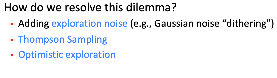
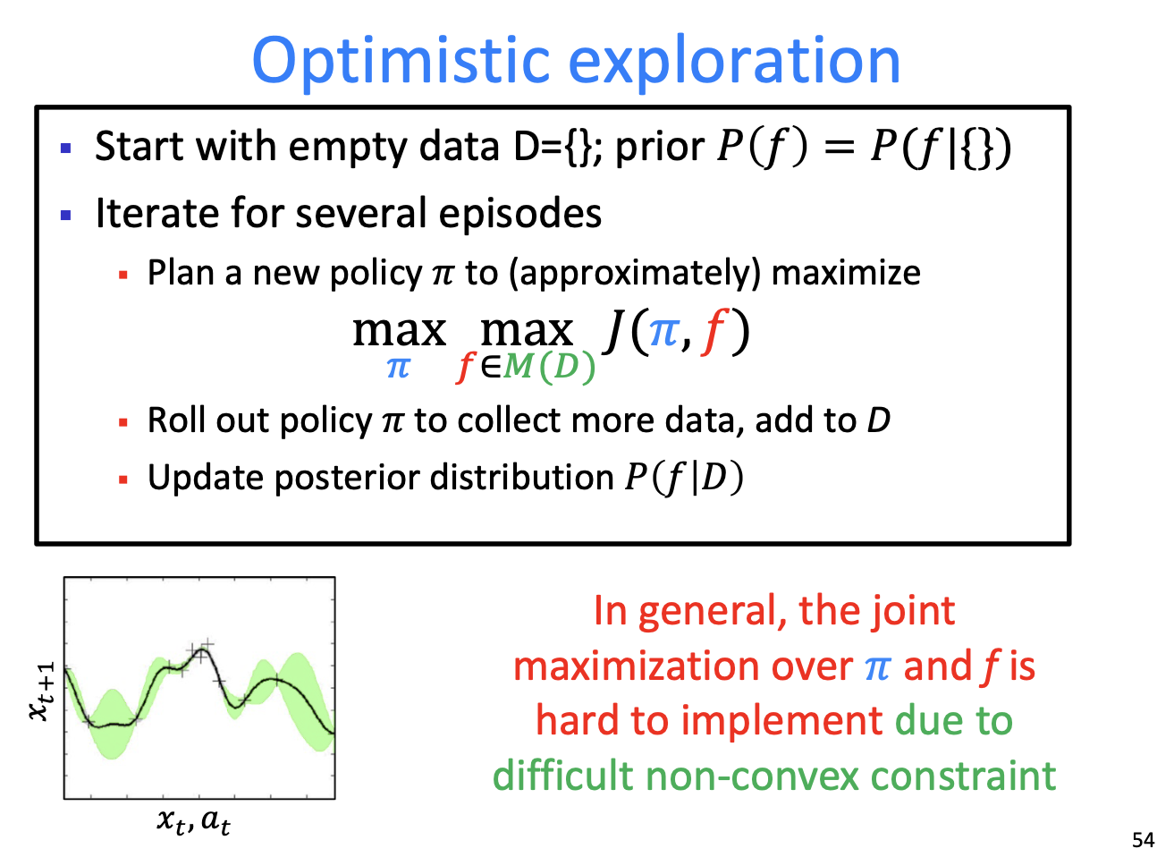
Thompson sampling
As in BO:
Optimism