Markov Decision Processes
Contents
A Markov Decision Process (MDP) is a mathematical model for sequential decision making under uncertainty.
The formal definition of a finite MDP is:
A finite MDP is specified by:
- a finite set of states \(X\);
- a finite set of actions \(A\);
- an initial state distribution \(P_0\);
- transition probabilities \(P(x' \mid x, a)\);
- a reward function \(r(x, a)\).
In the MDP setting we assume that we know \(P\) and \(r\), which is why we say it is a known environment, fully observable.
Goal: learn how the agent should behave to optimize its reward. How do we optimally decide what the next action is? This decision map is called a policy:
A policy is a function that maps each state \(x \in X\) of the MDP to a probability distribution over the actions:
\(\pi(a \mid x) = P(A_t = a \mid X_t = x), \quad t \geq 0.\)
For MDPs, optimal policies can always be taken to be deterministic. Interestingly, a policy induces a Markov Chain \(\{X^{\pi}_t\}_{t \in \mathbb{N}_0}\) with transition probabilities:
\[p^{(\pi)}(x' \mid x) = P(X^{\pi}_{t+1} = x' \mid X^{\pi}_{t} = x) = \sum_{a \in A} \pi(a \mid x)\, p(x' \mid x, a).\]So if the agent follows a fixed policy, the evolution of the process is described entirely by a Markov Chain.
But, as mentioned above, the goal is to maximise the reward — how do we do that? There are many ways. If we know the MDP (we can evaluate it for all \(a, x'\)), a very common choice is the discounted payoff. We want to maximise \(\mathbb{E}\!\left[\sum_{t=0}^{T-1} r(x_t, a_t)\right]\), discounted by a factor \(\gamma \in [0, 1)\), the discount factor. The discounted payoff from time \(t\) is the random variable
\[G_t = \sum_{m=0}^{\infty} \gamma^{m} R_{t+m},\]also called the infinite-horizon discounted reward.
Now we want to understand the effect of the initial state and initial action on the optimisation objective \(G_t\). To do so we use two functions:
- State-value function: expected return starting in \(x\) and following \(\pi\): \(v^{\pi}_t(x) = \mathbb{E}_{\pi}[G_t \mid X_t = x]\).
- State–action value function: expected return starting in \(x\), taking action \(a\), then following \(\pi\): \(q^{\pi}_t(x, a) = \mathbb{E}_{\pi}[G_t \mid X_t = x, A_t = a]\).
Above we considered deterministic policies; for a randomised policy we have \(\pi : X \to \Delta(A)\), mapping states to distributions over actions.
Computing the value of a policy: Bellman expectation equation
A policy is associated with its value function. How do we compute it? Recall:
\[J(\pi) = \mathbb{E}\!\left[r(x_0, \pi(x_0)) + \gamma\, r(x_1, \pi(x_1)) + \gamma^2 r(x_2, \pi(x_2)) + \cdots\right].\]Then
\[\begin{aligned} V^{\pi}(x) &= J(\pi \mid X_0 = x) \\ &= \mathbb{E}\!\left[\sum_{t=0}^{\infty} \gamma^t r(x_t, \pi(x_t)) \,\Big|\, X_0 = x\right] \\ &= r(x, \pi(x)) + \gamma \sum_{x'} p(x' \mid x, \pi(x))\, V^{\pi}(x'). \end{aligned}\]This is the Bellman expectation equation, and it shows the recursive dependence of the value function on itself: the value of the current state equals the immediate reward plus a discounted sum of all future rewards from subsequent states.
In vector form:
\[V^{\pi} = (I - \gamma P^{\pi})^{-1} r^{\pi}.\]This is a linear system, and solving it directly involves matrix inversion, which is cubic in time. There are faster ways:
Fixed-point iteration
Obtain an (approximate) solution to \(V^{\pi}\).
See notes and proof.
Policy optimization
Recall that our goal was to find an optimal policy:
\[\pi^{*} = \operatorname{argmax}_{\pi}\, \mathbb{E}_{\pi}[G_0].\]We can alternatively characterise an optimal policy via
\[\pi \geq \pi' \iff v^{\pi}(x) \geq v^{\pi'}(x), \quad \forall x \in X.\]It follows that all optimal policies have identical value functions; we write \(v^{*} = v^{\pi^{*}}\) and \(q^{*} = q^{\pi^{*}}\) for the value and action-value functions of an optimal policy. Then
\[v^{*}(x) = \max_{\pi}\, v^{\pi}(x), \qquad q^{*}(x, a) = \max_{\pi}\, q^{\pi}(x, a).\]We define the greedy policy with respect to a state–action value function as
\[\pi_q(x) = \operatorname{argmax}_{a \in A}\, q(x, a).\]Bellman optimality equation
Following the greedy policy \(\pi_v\) leads to a new value function \(v^{\pi_{v}}\). The correspondence between greedy policies and value functions induces a cyclic dependency:
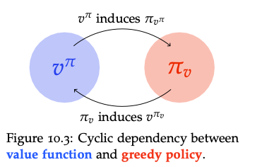
It turns out that the optimal policy \(\pi^{*}\) is a fixed point of this dependency. Hence:
A policy \(\pi^{*}\) is optimal iff it is greedy with respect to its own value function. Equivalently, \(\pi^{*}\) is optimal iff \(\pi^{*}(x)\) is a distribution over \(\operatorname{argmax}_{a \in A} q^{*}(x, a)\).
The optimal value function \(v^{*}\) is a fixed point of the Bellman update:
\(v^{*}(x) = \max_{a \in A} \big[\, r(x, a) + \gamma\, \mathbb{E}_{x' \mid x, a}[\, v^{*}(x')\, ]\, \big].\)
Policy iteration
See notes. Using the above we can converge faster than fixed-point iteration.